EnergyNet x ComboCurve: End-to-End Deal Evaluation Delaware Basin
We're using ComboCurve to highlight different assets the EnergyNet team brings to market. Take a look at Dylan Breaux’s end-to-end deal evaluation workflow of a non-operated working interest in 8 wells in the Delaware Basin, beginning with importing the asset’s ARIES database into ComboCurve.
You can view this listing with EnergyNet here.
Video Transcript
Dylan Breaux (00:03):
Hello, Dylan Breaux here, ComboCurve Senior Technical Engineer I’m walking through the forest behind my house right now to film this introduction because our marketing team said it would be more engaging. I’m going to do a daily evaluation after this where we look at some non-operated working interest in eight wells, Delaware basin. It’s pretty sizable, so really excited. We’re going to generate some type curves, run economics. Stay tuned.
Okay, so we’ve got a good size deal today. This one is going to be end to end, so it’s going to be a long form video. So stick with me because we’re going to go through it in real time, mostly real time. We’re going to skip a few steps again to keep everyone engaged. So what we’re looking at is this is lot 1, 1, 9, 2, 3, 5 Delaware Basin, Chevron, non-op working interest opportunity on some Undr locations. So it’s eight horizontal wells. We’ve got before payout interest here and after payout interest. So we can definitely model that here in ComboCurve. So remember that for later.
(00:44):
They provided us some information on offset activity, obviously the CapEx information to apply, but really step-by-step. What we’re going to do, get our data in to create type curves for these wells. Get the data in forecast, said wells, generate type curve, and then apply economics. So let’s just jump right in. Obviously you have the ability to bring in any kind of data that you want. In my case, I’m going to bring in some s and p global IHS data. It’s actually already integrated into my ComboCurve, but if you don’t have any kind of integration, you can definitely bring it in by Excel, which is really easy. So that would be literally you just dragging and dropping what you download from your favorite data source, whether that be well database, IHS and varis. Really anything in the Excel like format that’s got year, month, the volumes, all the header data drag and drop into ComboCurve basically by clicking data import. And then that’s where you can pull in Aries, page two N and then anything else in CSV.
(01:58):
So what I did, because I’ve kind of already got my area of interest automatically pulled in, I’ve got all the Delaware basin, what I can do is in my project I’ve got like 20,000 Delaware basin wells. What I can do is jump on the map and look directly at this area that energy net has provided to us. This is the opportunity. Here’s the section township range, and here it is in ComboCurve. So what I can do is basically select this area and then even create a buffer around, it’s like a 10 mile buffer. So I’m going to grab every well within that 10 mile radius and then I’m going to kind of filter by landing zone. So I want to grab the wells landing zones that I’m interested in. So bone springs Wolf Camp, Wolf camp A. I want to find wells that actually have monthly production data and I can really use this to filter anything else that I want to churn through. But this is a good starting point. 700 wells. Let’s forecast and then generate our type curves.
(03:04):
So again, filter down to 700 wells roughly. Next step, let’s get some solid forecasts on those because we’re following SPWE guidelines to not only forecast the monthly volumes, but we also want to use the forecast when generating that best fit curve. So this is where the ComboCurve auto forecaster comes into play and makes things very useful to get an initial really solid curve on all my wells. So again, here’s the 10 mile radius around the drilling location with the landing zones that I’m interested in. And just to revisit down here is the a FE summary by well where I can see the different targeted formations that I need to generate type curves for. So it looks like three, the wolf Camp XY A and the third bone springs. So that’s what we’re going to do.
(04:02):
So step one forecast said wells, this is where I can open my really configurable auto forecaster, get a solid forecast on all my wells. What’s nice is that you can save configuration. So I’ve already got a New Mexico, Delaware Basin 2024 configuration that I like, but again, this is where I’ve set balance from my V factor and my effective decline to forecast those data points as I see fit. I’m looking at the last 60 months of data and we’ll just click run. We’ll see the auto forecasting is running. It should take just about a minute, but again, who wants to sit here for a minute? This is my moment, my Rachel rain moment where I reveal that, okay, I’ve already done the auto forecaster. Let’s just start digging in.
(04:53):
All of my wells are forecasted. Now it’s up to me to QC and make sure it got solid forecast and then I can move on to my type curve. Step next. So wells are forecasted, I can jump through this page here and kind of QC the forecast that I run. If I see one that I want to tweak and finagle, this is where I could click this check box that sends it to the editing bucket and that’s where I can make all my manual adjustments. Obviously have the ability to add every well into the editing bucket and forecast every single one of those manually. But again, nice to get a head start with the auto forecaster. Another way to kind of QC and understand your wells is to run a diagnostic report. And this is basically going to give you information on EORs Q volumes, even data on completion design if you have it in this sheet.
(05:43):
And then you can use some of these visualizations to understand your data set. So in my case, this is where I can see all the different EORs of the wells that I forecasted. So if I want to maybe understand what makes these EORs so large, all I have to do here is filter to them. And then now I can either check the box and manually adjust them or I can even click on them and see this is 1.2 M barrels looks like a B factor of one. I mean it looks just like a really solid well. So anyway, one way to kind of QC and understand your wells. This diagnostics plot can also help you understand how your forecasts relate to your actuals. So I ran it on the last six months of data. And so now I can see from a cum D standpoint, which wells need that extra attention, maybe that the forecasts are off. So I can see a lot of wells matching up really nicely between forecast and actuals. But maybe we need to grab these 35 or so out of the 700 that are overperforming at those, the adding bucket, and then adjust those so that way we know we’ve got a really solid base to generate our type curves in this area.
(07:05):
And again, y’all don’t want to see me manually edit 30 or so wells. I’ve already done a little bit of that anyway, but just to give you another visual, this is the editing page where you can make all those manual adjustments. You can rerun your auto forecast if you want to or rerun it through a different set of data points. But I can click manual here and then really change my B factor, change everything else. We’ve got the keyboard shortcuts as well to help you churn through these wells and get onto actually generate your type curves for your new wells.
(07:38):
So with that next step really is to generate our type curve. And remember, like I said, we have three to generate. So to kick off that process, it’s very similar to the filter process that I presented to y’all earlier. We’d referenced the 700 wells that we forecasted, and then it’s just really up to me to choose a target formation. So in this case, maybe I want to start off with the bone springs wells. So I just filtered down to just those bad boys. And then actually I need to go to landing zone, not target formation. I like that header better.
(08:24):
So yeah, I would choose bone springs and now I’ve got 78 wells to begin my type curve, which I’ve already got pulled up over here. So to walk you through the type curve process, and again, what’s really nice here is that we’re staying within ComboCurve. You’re not jumping from tool to tool. Importing exporting would be great is that if I’ve already done this pre-work, maybe I know this area already, I can jump into a type I’ve already created, update the data, rerun all this, and maybe you won’t have to do this every single time you get a deal through, you’ve got your public data continually updating and then you’re just off to the races. As soon as you get a list of APIs, paste them in there and you’re ready to go.
(09:15):
But to kick off the type curve process, we try to follow SPW monograph five. It’s still in the works, but really the steps to generating a type well would be continually bending the wells and choosing which wells are most appropriate for a type curve, normalize, and then fit to that data. So that’s kind of what each one of these tabs represent. So with these visualizations I’m enabled to, and again, this is really customizable, but in this case I’ve got total prop and per foot versus first production date. So I can say let’s just already remove some of these early life, early time completed wells. Those aren’t going to be really relevant to probably a well that would be drilled today. Let’s just get rid of those data points. I’ve got it colored by operator here. These are newborn wells, so it doesn’t look like they’ve drilled at least any bone springs wells to according to this public data at least. So that doesn’t really help us out, but good to have here. And again, I could use the probe it plot, use the map again to find outliers. Maybe I want to only find wells that are drilled north to south, like the ones that they’re going to be drilling that they proposed.
(10:37):
But we’ll just jump to the normalization section next. Again, this is where I can normalize based off of really any well header that I bring in, whether that be lateral length, prop per foot, fluid per foot, and then actually normalize several different ways, kind of that one-to-one fit double your per later length, double your EOR or these linear power loft fits. Actually use the equation to fit the fit through the data to understand that correlation and normalize correlation. And so I’ve already kind of got this preset, but this is really customizable. You can adjust your fit function manually or autofit it and then do the same for oil, gas, and water. And what’s really nice here, and I’ll show you this too, is that once we create these wells, if you input in the header data what the lateral length is, it will automatically normalize for you. So I’m not creating eight different type curves. I am creating just one and then normalizing based off of the lateral lengths that they propose. And then really the final section, again, similar to kind of the way I set the auto forecaster up to fit this wells average, which is using the monthly production data and the forecasted data, I can set bounds again for my B factor and my affected decline, choose several different multis segment fit types and then choose all of them for oil, gas, and water. But we’ll click run and very quickly you’ll see a dash line populate
(12:09):
Across this orange wells average line. You go, boom, I could toggle on the different P 10, P 50, P 90 here as well, and actually use those in my economics as well. So if somebody wanted to see that on the management side, you’ve got those run all three at one time because of the ability to run multiple scenarios at one time and you come in locked and loaded to present to your executives, but we’ll click save. We won’t do the other two type curves, but that’s one. Do that two more times and then jump to economics. Really the only probably steps, and I’ll just briefly show ’em to you, they’re not very exciting, but would be to create eight new wells made very easily by the create wells feature here under settings. I tell Comic Booker how many wells I want to create these wells are called the 49 er ridge unit. So I just give them a name and then I can actually tell it what headers I want to adjust. So like lateral length operator if I wanted to landing zone,
(13:20):
Oops, not that one landing zone. And then boom, I’ve got eight wells created. And then what’s awesome is that I’ve got this Excel spreadsheet in here very quickly I can just paste in. There are lateral links here, paste in landing zone, and boom, just like that. I’ve created eight wells, which I have already done. Again, I’m Rachel rang it a little bit. Last thing I’ll touch on too that I did for this last thing before economics that I’ll touch on is that I did actually create a schedule, just a really easy way to kind of build out a potential timing for these wells in the documentation. It said in the AFEs, it said they were planning for a Q3 2024 drill date. So basically what I did was I filtered down to those eight wells and then within the tool you can actually build this out completely what it looks like to drill a well.
(14:31):
So you could schedule in pad prep, drilling completion facility, do it on a sequential or do batch drilling, batch completing, and then toggle on and off how many completion crews and how many drilling units you would have and their availability. So it’s a way once you click run and I’ve already again pre ran, it just takes a couple minutes, but it will output this spreadsheet for you and it’ll give you information like first production date after you give it a program, start date, first production date drill, start, completion start, and then automatically your economics can tie to these dates. So it’s really easy to run a couple different scenarios. Who knows exactly when they’re going to drill these. Maybe it’s September, October, maybe it’s next year. Maybe it’s worth throwing one of those in there just in case you being a non-op, you don’t exactly have control. So it’s really easy to build out very quickly, a few different scenarios for this. And you can also visualize it in a Gantt chart form as well, which I really like helpful to present to management and showcase. We’re doing our due diligence buddy. So great, well scheduled type curves created wells, created final step, filter down to those eight wells and create a economic scenario.
(15:59):
And if y’all haven’t seen ComboCurves economic engine before, it’s laid up pretty differently than other platforms is actually in this tabular format. So each one of those wells, those 49 ER ridge units are represented here in these rows. And then your economic output or your economic models are going to be represented in these columns. So again, a couple of different ways you can apply economics, but one is very excel like and functionality. So as you can see here, it was very easy for me to export this table out to Excel and then paste it back in for things like my completion cost or my CapEx expenses here.
(16:42):
But what kind of work left to right. So I’m getting ahead of myself. Ownership, and this is something that I teased at the beginning of our walkthrough here, but what’s nice here is that you can schedule up to 10 different reversions. So remember back on our spreadsheet here, they talked about before payout after payout, working interest in NRI. This is where you can build that out. You have your initial working interest and then you can select from here, different types of reversions, revert on a certain date, IRR or payout in our case, and toggle on that different working interest in NRI for all your wells. What’s nice is these all have the same working interest in NRI. So just pasted it straight down here. I applied my different type curves based off of a lookup table, which if you haven’t used those before in you are a ComboCurve user, you got to reach out to your CS team and they can show you how to make your life a lot easier when dealing with some of these packages. I applied that drill schedule that we built. The as of date for this property or for this opportunity was 6 1 20 24. I applied the CapEx that they recommended based off of a Excel spreadsheet running through this a little bit. This is the least exciting thing is copy and pasting. It’s so easy is unexciting. Is that fair to say?
(18:08):
Finally, I applied a pricing here. I’ll show this because who doesn’t love a good easy price application? So this is where then ComboCurve, you can apply your flat assumptions if you like 70 oil, 1.8, 1.9 gas. You can do it in a time series. And then we also have these embedded price decks as well. So this pulls from the CME database where you can choose any date back in time. It’ll be the close of the brent crude IMEX WTI or the Henry hub, boom boom. And just like that, you’ve got your strip that you could use. And this is all really customizable as well. So if I wanted to paste in my own internals, I could do that here. But again, I use this to actually create a price model and then brought in the actuals because this is a backward dated, I guess, not that it matters because they’ve already been drilled. And then last thing would be expenses. And hey, maybe this is time for a call out to viewer here. I’m not a Delaware expert, I’m not an expert in anything really. So this is what I used for my expenses. I just have a fixed expense and then a water disposal cost in time series. I’ve got 12 months of 9,000, then it goes down to 65, and then four, maybe I’m way off base, maybe I’m a little low, curious what y’alls thoughts post below in the comments.
(19:45):
And then finally, we’ve applied production Texas, but enough about boring all economics. The final step now would be to click run scenario. This is where most importantly, you go to the combo section and you’re able to run multiple different economic scenarios. So if you want to go to your management team and show them three different price assumptions or three different schedules or CapEx assumptions or risk it, this is where you can build that out and have 10 different economic parameters at one time. Sorry, up to 10. I just showed you three. And so then finally, I actually haven’t even hit run, so I need to do that.
(20:33):
Okay, unpause, I ran economics three runs on these eight wells. It took less than a minute to run three economic runs on these well, so really didn’t even have to pause. But anyway, now I’ve got my three different runs on price. But again, this could be on schedule, this could be on CapEx assumptions, really anything. And then from there, it’s really ready. It’s time for me to consume, make a decision, get everything ready to present to management. Yay or nay, let’s purchase this. Or if I’m managing myself, then act even quicker. But to do that, there’s this custom PDF editor that’s relatively new that we’re pretty excited about. But this is where two be able to present the management or banks for anybody. You want clear and concise data. And so we have this nice little skeleton template here to where I can put exactly what I want in this report to send out.
(21:39):
You don’t want to overwhelm anybody with information. So let’s only put IRR payout rate of return, only X amount of discount cash flows, rollups, put in landscape mode, throw doing logo up there to look really professional. And again, that’s for all your different economic runs. So 10 different ports and then you’re off to the races. But that really wraps about it. That was end to end. We’re at the end now I think in the script, supposed to call to action. So that action is, hey, reach out, teach me a little something about the Delaware basin. Comment below or other call to action. Go on energy net, check out this deal. Check out other deals. There’s lots of exciting opportunity to be had out there. This is Dylan, Breaux, signing off.
See how your team can go from forecast to economics in minutes with energy’s fastest analysis engine.
Related Posts

The State of GHG Emissions Planning in Oil and Gas
Even the most ambitious energy transition plans still include the production and consumption of significant amounts of oil and gas until 2050 and beyond.

Three Reasons Oil & Gas Companies Are Planning for Net-Zero
Reduce exposure to regulations, create transparent future emissions forecasts to attract capital, and enable a balanced mix of sustainable energy sources.
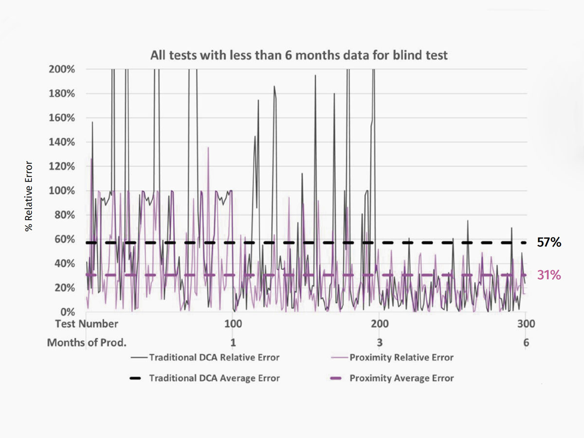
ComboCurve Proximity vs. Traditional DCA Forecast: A Comprehensive Comparison Study
ComboCurve’s proximity workflow generates a forecast with a much lower error compared to the traditional DCA.